Getting Started with UncertainSCI
System Requirements
Requires Python 3 and modules listed in requirements.txt
Getting UncertainSCI
The easyiest way to get UncertainSCI is to use pip. Just run pip install UncertainSCI or python -m pip install UncertainSCI and pip will download and install the latest version of UncertainSCI. This will also try to download and install the relevent dependencies too.
To get pip, see its documentation.
The source code for UncertainSCI can be downloaded from the Github page.
Installing UncertainSCI From Source
UncertainSCI can be built from source code using the setup.py script. To call this script, navagate to the source root directory in a terminal window and run the command pip install . or python -m pip install .
UncertainSCI Overview
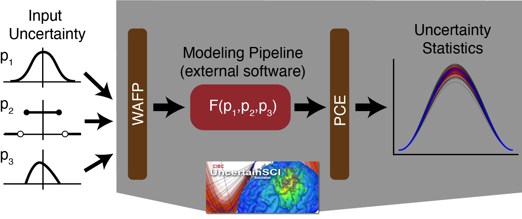
Users can evaluate the effect of input uncertainty on forward models with UncertainSCI’s implementation of polynomial Chaos expansion (PCE). The pipeline for the process is shown in the following image:
Before Using UncertainSCI
In order to run UncertainSCI, it must be supplied with the input parameter distributions, a model that will run the parameters in question, and a way to collect model solutions for use in PCE. The model itself can be implemented in Python or in another software, as appropriate, as parameter sets and solutions can pass between UncertainSCI and modeling software via hard disk. Models with high resolution solutions should could be cost prohibitive to run with PCE, so users should consider derived metrics or solutions subsets (regions of interest) for UQ.
Users must chose the input distributions for their modeling pipeline, which may significantly impact the output distributions. The indendent application will determine the best distributions to use, yet we suggest that the users use all information available to inform their choices. Published literature and previously generated data are, of course, more credible, but users may need to rely on their own intuition and observed trends with the targeted model.
PCE computation time
Since UncertainSCI uses PCE to compute UQ, it is worth noting the impact of some PCE parameters on computational time. Mostly, the time needed to compute UQ via PCE is limited by the evalutated model, especially in bioelectric field and other 3D simulation applications. PCE attempts to reduce computational cost by limiting the number of parameter samples are needed to estimated the model output distributions, as the fewer parameter sets needed, the few times the model needs to be run. Since PCE is estimating a polynomial to represent the output distribution, some user choices will affect the sample size
Number of parameters modeled in the PCE will affect the number of samples needed to estimate the model uncertainty by increasing the dimensionality of the estimated polynomial. Higher demensions require more sampling points to accurately capture, so will lead to higher computation times. However, parameters must be evaluated in the PCE together to determine the effect of their interaction in the targeted model.
polynomial (PCE) order affects the PCE samples needed for UQ by defining the complexity captured by PCE. As in 1D, polynomials with higher order are able to capture higher variability within the domain. Therefore, models with high complexity, i.e., significant response to variation in the parameter space, should use higher polynomial orders. However, more parameter samples are required to estimate higher polynomials, increasing the number of times the model must be run.
Distribution type of the parameters may effect the number of samples, but to a minor level when compared to number of parameters and polynomial order.
Running UncertainSCI
Running UncertainSCI for Sample Generation
With the model setup, the user will need to setup the input parameter distribution using UncertainSCI’s distribution datatype. While there are a few distribution types to choose from, the Beta distribution is a common choice. If we had three input parameters, we can define a different beta distribution for each, thus:
from UncertainSCI.distributions import BetaDistribution

Nparams = 3
# Three independent parameters with different Beta distributions
p1 = BetaDistribution(alpha=0.5, beta=1.)
p2 = BetaDistribution(alpha=1., beta=0.5)
p3 = BetaDistribution(alpha=1., beta=1.)
For the default case used in here, the range of each parameter is [0 , 1].
After the input parameters are set, we can generate a parameter sampling that will most efficiently estimate the UQ. In order to do this, the user must create a PCE object with the distributions. However, the user must also define a polynomial order. This defined as an integer:
# # Polynomial order
order = 5
Now we can create the PCE object and generate parameter samples:
from UncertainSCI.pce import PolynomialChaosExpansion

# Generate samples first, then manually query model, then give model output to pce.
pce = PolynomialChaosExpansion(distribution=[p1, p2, p3], order=order, plabels=plabels)
pce.generate_samples()
To use the samples generated by this PCE instantiation, users can access it through the object:
import numpy as np # output is np array
pce.samples
Which returns a numpy array of size MxN where N is the number of parameters and M is the number of samples (determined by uncertainSCI).
Running Parameter Samples for Model Outputs
While this is heavily dependent on the modeling pipeline, the generated samples can be save to disk to run in an external pipeline:
np.savetxt(filename,pce.samples)
or called within python:
for ind in range(pce.samples.shape[0]):
    model_output[ind, :] = model(pce.samples[ind, :])
If the samples are saved to disk to run asyncronously, they will need to be added to a PCE object if the original one is destroyed. This happens when it is run as a script, then rerun with data and is acheived with:
pce.set_samples(np.loadtxt(filename))
instead of running pce.generate_samples(). Similarly, the output results from the simulation will need to be a numpy array of MxP where M is the number of parameter sets, and P is the size of the solution array. 2D and 3D solutions can be flattened into a 1D array and collated into this solution array, then reshaped for visualization.
PCE and the Output Statistics
With the appropriate distributions and samples added to the PCE object and model output collect, the estimator and output statistics can be generated. First, the PCE must be built:
pce.build(model_output=model_output)
Then, output statistics can be return:
mean = pce.mean()
stdev = pce.stdev()
global_sensitivity, variable_interactions = pce.global_sensitivity()
quantiles = pce.quantile([0.25, 0.5, 0.75]) #  0.25, median, 0.75 quantile
There are also built in ploting functions (with matplotlib) for 1D data:
from matplotlib import pyplot as plt
mean_stdev_plot(pce, ensemble=50)
quantile_plot(pce, bands=3, xvals=x, xlabel='$x$')
piechart_sensitivity(pce)

plt.show()
The API documentation explains the implementation of UncertainSCI in more detail.
Running UncertainSCI Demos
There are a number of demos included with UncertainSCI to test it’s installation and to demonstrate its use. The previous description can be found as a notebook with some more details here and as a script in demos/build_pce.py.
The demo scripts can be a way to quickly test the installation. Make sure that UncertainSCI is installed, then simply call the script with python using the command python demos/build_pce.py. Other demos can be run similarily.
We have included a number of demos and tutorials to teach users how to use UncertainSCI with various examples.