Simple Example Showing UQ With PCE

This example shows some basic functionality of UncertainSCI using the polynomial Chaos emulators (PCE) to quantify uncertainty in a 1D function. It is essentially identical to demos/build_pce.py and uses a 1D Laplacian ODE as a model with three parameters

import numpy as np
from matplotlib import pyplot as plt

from UncertainSCI.distributions import BetaDistribution
from UncertainSCI.model_examples import laplace_ode_1d
from UncertainSCI.pce import PolynomialChaosExpansion

from UncertainSCI.vis import piechart_sensitivity, quantile_plot, mean_stdev_plot

Model Parameter setup

The first step in running UncertainSCI is to specify the parameter distributions and the capacity of the PCE model (polynomial order).

Distributions

# Number of parameters
Nparams = 3

# Three independent parameters with different Beta distributions
p1 = BetaDistribution(alpha=0.5, beta=1.)
p2 = BetaDistribution(alpha=1., beta=0.5)
p3 = BetaDistribution(alpha=1., beta=1.)

plabels = ['a', 'b', 'z']

Polynomial Order

How complicated the model is

# # Polynomial order
order = 5

Forward Model

\[-\frac{d}{dx} a(x,p) \cdot \frac{d}{dx} u(x,p) = f(x)\]

with \(x\) in \([-1,1]\) discretized with \(N\) points, where \(a(x,p)\) is a Fourier-Series-parameterized diffusion model with the variables \(p_j=[a, b, z]\). See the laplace_ode_1d method or UncertainSCI/model_examples.py for details.

N = 100
x, model = laplace_ode_1d(Nparams, N=N)

Running PCE in UncertainSCI

The steps to running PCE in UncertainSCI are - create PCE object - generate parameter samples - run parameter sets in the forward model - give model output to PCE - compute output statistics

Create PCE object and Build Sample Set

With the parameter distribution created and polynomial order set, we can create the PCE object and generate a parameter set that will efficiently and accurately estimate the output distribution of the model. UncertainSCI adds an extra 10 parameter sets as a precaution.

pce = PolynomialChaosExpansion(distribution=[p1, p2, p3], order=order, plabels=plabels)
pce.generate_samples()

print('This queries the model {0:d} times'.format(pce.samples.shape[0]))

Precomputing data for Jacobi parameters (alpha,beta) = (-0.500000, 0.000000)...Done
This queries the model 66 times

Run Parameter Sets in the Forward Model

We query each parameter set in sequence to run in our Laplacian ODE model and collect the results

model_output = np.zeros([pce.samples.shape[0], N])
for ind in range(pce.samples.shape[0]):
    model_output[ind, :] = model(pce.samples[ind, :])

Build PCE from Model Outputs

With the collated model solutions, the output distributions can be estimated using PCE

pce.build(model_output=model_output)

array([1.75571628e-37, 5.64860235e-17, 2.10743598e-16, 4.30180091e-16,
       6.73615485e-16, 8.98426649e-16, 1.06808811e-15, 1.15833221e-15,
       1.16057868e-15, 1.08209494e-15, 9.43231789e-16, 7.72726181e-16,
       6.02299430e-16, 4.61625174e-16, 3.74362183e-16, 3.55551159e-16,
       4.10403164e-16, 5.34387196e-16, 7.14489737e-16, 9.31478341e-16,
       1.16290358e-15, 1.38643597e-15, 1.58302359e-15, 1.73934375e-15,
       1.84914225e-15, 1.91328322e-15, 1.93860602e-15, 1.93592175e-15,
       1.91761943e-15, 1.89536658e-15, 1.87829599e-15, 1.87191182e-15,
       1.87777401e-15, 1.89387162e-15, 1.91549769e-15, 1.93639635e-15,
       1.94995954e-15, 1.95029022e-15, 1.93300605e-15, 1.89571844e-15,
       1.83817752e-15, 1.76211869e-15, 1.67087823e-15, 1.56886365e-15,
       1.46096875e-15, 1.35201633e-15, 1.24629417e-15, 1.14722754e-15,
       1.05720583e-15, 9.77557484e-16, 9.08648189e-16, 8.50065649e-16,
       8.00849025e-16, 7.59724059e-16, 7.25312441e-16, 6.96294722e-16,
       6.71517851e-16, 6.50048858e-16, 6.31183955e-16, 6.14427000e-16,
       5.99452329e-16, 5.86065283e-16, 5.74169862e-16, 5.63747820e-16,
       5.54848130e-16, 5.47581156e-16, 5.42108762e-16, 5.38620514e-16,
       5.37288102e-16, 5.38194279e-16, 5.41239598e-16, 5.46038218e-16,
       5.51822165e-16, 5.57379403e-16, 5.61052914e-16, 5.60824129e-16,
       5.54493189e-16, 5.39951481e-16, 5.15520386e-16, 4.80308188e-16,
       4.34519740e-16, 3.79646212e-16, 3.18469931e-16, 2.54843985e-16,
       1.93246402e-16, 1.38157999e-16, 9.33612879e-17, 6.12921066e-17,
       4.25845893e-17, 3.59260824e-17, 3.82825975e-17, 4.54770963e-17,
       5.30202417e-17, 5.70278062e-17, 5.50298773e-17, 4.64948566e-17,
       3.29537537e-17, 1.77021507e-17, 5.15427668e-18, 0.00000000e+00])

Compute Output Statistics

With the PCE built, statistics can be calculated for each point in the solution space (x).

## Postprocess PCE: statistics are computable:
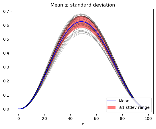
mean = pce.mean()
stdev = pce.stdev()
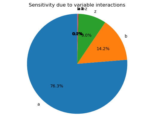
global_sensitivity, variable_interactions = pce.global_sensitivity()
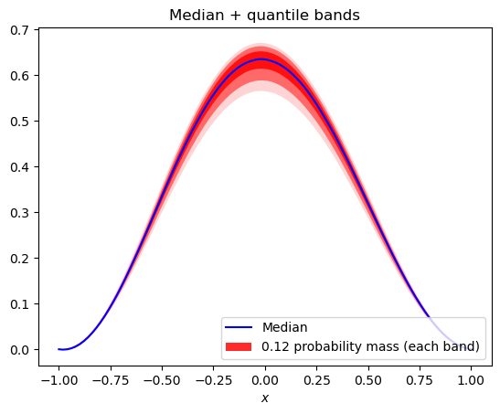
quantiles = pce.quantile([0.25, 0.5, 0.75]) #  0.25, median, 0.75 quantile

Output Visualizations

To help understand and interpret UQ statistics, we’ve included some plotting tools for 1D data.

mean_stdev_plot(pce, ensemble=50)

<AxesSubplot:title={'center':'Mean $\\pm$ standard deviation'}, xlabel='$x$'>

quantile_plot(pce, bands=3, xvals=x, xlabel='$x$')

<AxesSubplot:title={'center':'Median + quantile bands'}, xlabel='$x$'>

piechart_sensitivity(pce)

<AxesSubplot:title={'center':'Sensitivity due to variable interactions'}>